Implementing Different Types of RL Models
Note: This post will be updated as I implement different types of RL models. Code can be found here: https://github.com/vulcan-332/deep_rl
The purpose of this post is to implement different RL algorithms in code, going beyond theory. The examples will focus on simple environments to make it easier to understand the inner workings of the algorithms. For speeding up the setup, environments are pre-built and imported from Gymnasium1. For the theoretical background, 2 and 3 are some great sources to begin with.
You can use any package manager, I will be using conda. Basic packages are numpy, matplotlib, and gymnasium.
conda create -n deep_rl python=3.10
conda activate deep_rl
pip install gymnasium
pip install matplotlib
Q-Learning
Q-Learning is a Model-Free, Value-Based algorithm. This means the agent doesn’t need to know the environment’s physics; it only needs to estimate the value (expected future reward) of taking a specific action in a specific state. The environment used for this Q-learning project is the FrozenLake grid world, but crucially, it is configured to be non-slippery (deterministic). This means that when the agent chooses an action (Up, Down, Left, or Right), it executes that move with 100% certainty. The environment is a simple 4x4 grid where the agent must navigate from the starting point (S) to the goal (G) while avoiding fatal Holes (H) 4.
gymnasium.make("FrozenLake-v1", is_slippery=False).

The brain of our agent is the Q-Table (represented in our code as a Python defaultdict). This table stores the Q-Value for every possible State-Action pair, $Q(s, a)$.
State ($s$): The agent’s current location or configuration.
Action ($a$): A move the agent can take (e.g., Up, Down, Left, Right).
Q-Value: The estimated maximum discounted future reward for taking action $a$ in state $s$.
The agent continuously updates its Q-Table based on the results of its actions. The update is driven by the Temporal Difference (TD) Error, which measures the difference between the agent’s expected value and the value it actually observed. The basic update rule for the q-value table is as follows:
\[\text{New } Q(s,a) \leftarrow Q(s,a) + \alpha \cdot [\underbrace{(r + \gamma \max_{a'} Q(s', a'))}_{\text{TD Target (Observed Reality)}} - \underbrace{Q(s,a)}_{\text{Current Estimate}}]\]where $\alpha$ is the learning rate - how quickly the agent replaces old knowledge with new information (e.g., 0.3) and $\gamma$ is the discount factor - how much the agent values future rewards versus immediate ones (e.g., 0.99).
For example, if the agent is in state $S_1$ and takes action $move_right$, it receives a reward $0$ and transitions to state $S_2$. The agent then updates its Q-Value for the state-action pair $(S_1, move-right)$ based on the TD target and TD error.
This TD target is calculated as follows:
\[\text{TD target} = (r + \gamma \max_{all-actions}(Q(S_2, all-actions)))\]where $r$ or (0) is the reward received, $\gamma$ is the discount factor (0.99), $S_2$ is the next state, and $move-down$ is the best action in the next state.
And consequently, the TD error is calculated as follows:
\[\text{TD error} = \text{TD target} - Q(S_1, move-right)\]Finally, the next q-value is calculated as follows:
\[\text{New } Q(s,a) \leftarrow Q(s,a) + \alpha \cdot [\text{TD error}]\]The core challenge for any RL agent is deciding whether to try a new path (Exploration) or follow the best-known path (Exploitation). We solve this using the $\epsilon$-Greedy Policy. At every step, the agent performs a coin flip governed by the variable $\epsilon$.
Exploitation (If random number $\ge \epsilon$): The agent chooses the action with the highest Q-value using argmax. This is the greedy choice action = np.argmax(qs)
Exploration (If random number $< \epsilon$): The agent chooses a random action, potentially discovering a better, faster, or safer route action = env.action_space.sample().
To ensure the agent converges, we start with a high $\epsilon$ (1.0) and slowly reduce it over time (epsilon_decay = 0.995). This forces the agent to transition from purely random exploration at the start to highly confident exploitation at the end. The training variance we observed early on was a direct result of the agent desperately trying to find the first reward while $\epsilon$ was still high.
The core loop of Q learning is as follows:
np.random.seed(42)
episodes = 5000
reward_history = []
Q = defaultdict(float)
gamma = 0.99
alpha = 0.3
epsilon = 1.0
epsilon_min = 0.05
epsilon_decay = 0.995

for ep in range(episodes):
    state, info = env.reset()
    done = False

    while not done:
        # --- 1. Choose Action (Epsilon-Greedy) ---
        if np.random.rand() < epsilon:
            action = env.action_space.sample() # Explore
        else:
            # qs is a list of Q-values for all actions in the current state
            qs = [Q[(state, a)] for a in range(env.action_space.n)]
            action = np.argmax(qs) # Exploit

        next_state, reward, terminated, truncated, info = env.step(action)
        done = terminated or truncated

        # --- 2. Calculate TD Target ---
        best_next_q = max(Q[(next_state, a)] for a in range(env.action_space.n))
        # (1 - done) ensures the Q-value is 0 if the episode terminated
        td_target = reward + gamma * best_next_q * (1 - done)

        # --- 3. Update Q-Table ---
        td_error = td_target - Q[(state, action)]
        Q[(state, action)] += alpha * td_error

        state = next_state

    # Epsilon decay occurs after the episode ends
    epsilon = max(epsilon_min, epsilon * epsilon_decay)
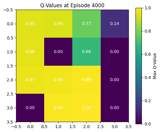
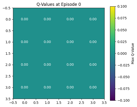
The Q-values represent the agent’s estimated maximum total future discounted reward it can obtain by taking a particular action from a given state. At the very beginning of training, the agent has no experience. It has no estimate of which states are good or bad, so the expected future reward from any state is zero. Based on the image from the final Q-Values, this time, the agent has learned the optimal policy. The heatmap now shows, for each state, the maximum Q-value over its possible actions. Higher values indicate states from which the agent expects to obtain high future rewards by behaving optimally. It starts off at 0.95 in the top right ((0,0) where the agent begins) and increases as the agent gets closer to the goal (3,3). The states where there are holes are marked with a value of 0.0 because the agent has learnt that the simulation ends without a reward if it steps into a hole. The state right before the goal has a q value of 1, because reward can be immediate if the agent takes the optimal step. The goal state itself has a value of 0.0 in the Q-table visualization. This is not because the agent believes the goal is bad, but because the episode ends immediately upon entering the goal, so there are no actions to take and therefore no future rewards to estimate. Thus, the Q-values for the terminal (goal) state remain zero, even though reaching that state is the correct objective.