Engineering a Tiny World Model: Representation, Latent Dynamics, and Rollout Stability
Project Repository: https://github.com/vulcan-332/latent_dynamics
Introduction
World models are appealing because they promise something simple and powerful: instead of reacting only to the current observation, an agent can learn an internal simulator of the environment and use that simulator to imagine the future.
The most recent push with JEPA 1, V-JEPA 2 2, and earlier latent world-model work such as World Models 3 and PlaNet-style latent dynamics 4 argue that true intelligence can be achieved not through language, but by understanding interactions of any two systems.
That idea shows up everywhere now, in model-based reinforcement learning, robotics, video prediction, and latent planning. But in practice, “I trained a world model” can mean very different things. A model that reconstructs frames well is not necessarily a model that can predict future states well. A model that predicts the next step well is not necessarily a model that can roll out ten steps without drifting off course.
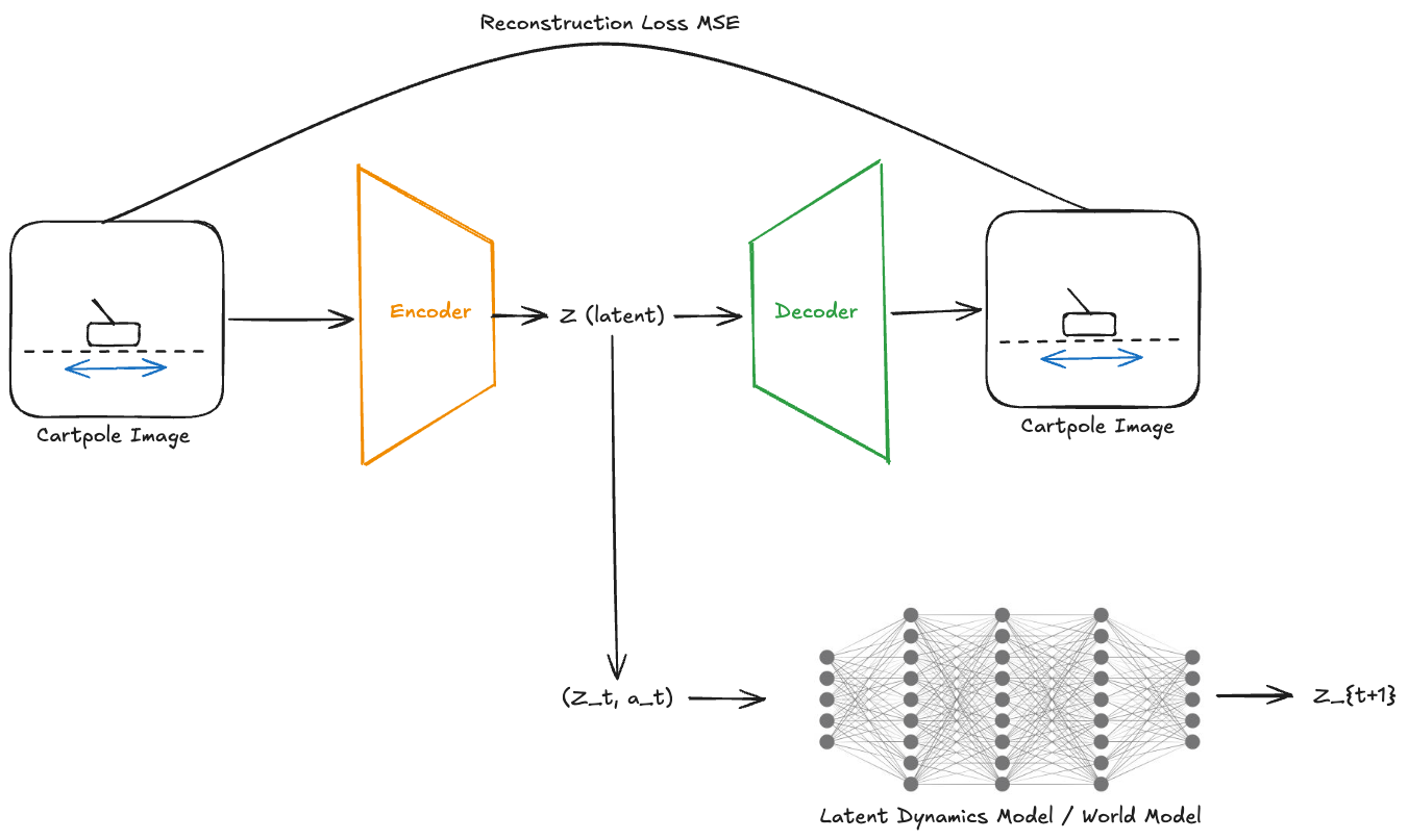
In this post, I built a small “world model” for CartPole from pixels and evaluated it in the simplest way I could think of. The final system has three parts:
- an encoder-decoder that maps frames to a latent state
z, - a latent dynamics model that predicts the next latent state from the current latent and action,
- a set of evaluation experiments to answer a practical question:
Is the learned latent state actually useful for control, and how accurate does the world model stay when rolled forward over time using its own predictions?
The answer, as usual, is: partly yes, and only if you measure the right thing.
Why this project?
CartPole is a toy RL environment, but it is useful precisely because it is small enough that failure modes are easy to interpret.
The environment already provides the true underlying state:
- cart position
- cart velocity
- pole angle
- pole angular velocity
If the goal were purely to solve CartPole, I would just use those four numbers. But that is not what world models are for. The point here is to start from rendered frames, learn a compressed internal representation, and ask whether that learned representation behaves enough like “state” to support prediction and control.
That makes CartPole a good microscope:
- simple enough to build end-to-end,
- structured enough that representation errors are visible,
- small enough that qualitative debugging still matters.
The system
The project has two separate learning problems:
- Representation learning
Learn a latent state $z_t$ from the image $x_t$.
- Dynamics learning
Learn how that latent changes when an action is applied:
\[(z_t, a_t) \xrightarrow{M} z_{t+1}\]Once both parts are trained, the system can “imagine” future latent states by repeatedly applying the dynamics model (M). That is the core world-model loop.
Step 1: Collecting data from the environment
I first rolled out CartPole with a random policy (select random actions $a_t$) and stored transitions of the form:
$(x_t, a_t, x_{t+1}, r_t, done_t)$
where $x_t$ and $x_{t+1}$ are rendered frames. This gave the model info about how a random action changes the state.
A practical detail that mattered immediately
Raw CartPole frames are mostly blank white background. If you train directly on those, the model can get low reconstruction loss by learning background statistics while paying relatively little attention to the thin pole itself.
So I added two preprocessing choices:
- crop the frame to focus on the cart/pole region,
- convert to grayscale.
That made the representation problem much better behaved. This was one of the first lessons of the project: in visual environments, preprocessing can matter more than architecture.
Step 2: Learning a latent representation
The first model is an autoencoder:
encoder $E(x_t) \to z_t$
decoder $D(z_t) \to \hat{x}_t$
trained with reconstruction loss ${L}_{rec} = |x_t - \hat{x}_t|^2$
The goal at this stage is not “planning” or “control.” It is simply to answer: Can I compress a frame into a latent code and still reconstruct the important parts of the scene?
The answer was yes. The reconstructions were clearly recognizable CartPole frames. That gave me a latent representation z that I could treat as the internal state of the world model.
The next question then becomes: Does this latent representation vector contain enough information to let a dynamics model know the state of the system i.e, the pole angle and the cart position.
Step 3: Learning latent dynamics
Once frames were encoded into latents, I trained a dynamics model M : \((z_t, a_t) \xrightarrow{M} z_{t+1}\) using a simple MLP.
The input was:
- latent state $z_t$
- one-hot encoded action $a_t$
The target was the latent of the next frame, $z_{t+1}$
This is the simplest possible latent dynamics model. No recurrence, no transformer, no latent stochasticity. Just a feedforward predictor.
Defintion of state
A true state in control is supposed to be Markov: it contains enough information to predict the future. That becomes important later. A single image frame often gives you:
- cart position,
- pole angle,
but not perfectly:
- cart velocity,
- pole angular velocity.
So even before any experiments, there was already a likely weakness in the setup: a single-frame latent might reconstruct well, yet still be incomplete for dynamics.
Evaluation 1: Can a controller learn from the latent state?
Before asking whether the world model can imagine the future, I wanted to ask a simpler question:
Does the latent state contain enough information to support control at all?
To test this, I trained two controllers with the same architecture:
Controller A: trained on the true environment state $[x, \dot{x}, \theta, \dot{\theta}]$
Controller B: trained on the learned latent state $z$
Both controllers were trained to imitate the same simple expert rule.
At first I used a rule based on both angle and angular velocity, but that turned out to make the comparison unfair because a single image does not reliably expose velocity. So I simplified the target policy to depend only on the sign of the pole angle.
That made the question much cleaner:
If the action depends mostly on angle, can a network trained on z recover the same policy nearly as well as a network trained on the true state?
Result:
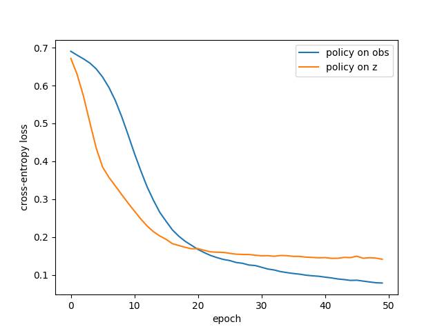
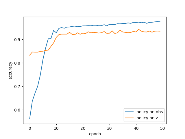
The policy trained on the true observation vector learned faster and reached higher final accuracy. The policy trained on z also learned well, but plateaued slightly worse.
That is exactly the result to expect because the observation vector is:
- low-dimensional,
- noise-free,
- directly provided by the simulator,
- almost a best-case control input.
The latent z is:
- learned from pixels,
- compressed,
- influenced by cropping and reconstruction choices,
- a noisier proxy for the actual state.
So the right goal was never for z to beat the true state. The right goal was for z to get close enough to be useful, which it did.
Tracking both loss and accuracy
Cross-entropy loss and accuracy do not tell the same story. A classifier can be mostly correct but not very confident. In my experiments, that is exactly what happened: the latent-based policy achieved high accuracy, but its loss stayed higher than the obs-based policy.
That means the latent controller was often correct, but less certain. That is a useful distinction. It says that the representation contains the right information often enough, but the decision boundary in latent space is messier than in the true state space.
Evaluation 2: One-step prediction vs multi-step rollout
A world model that predicts the next step accurately is only useful locally. What really matters for imagination is whether it can be rolled forward repeatedly without drifting.
To separate those two questions, I used two evaluation modes.
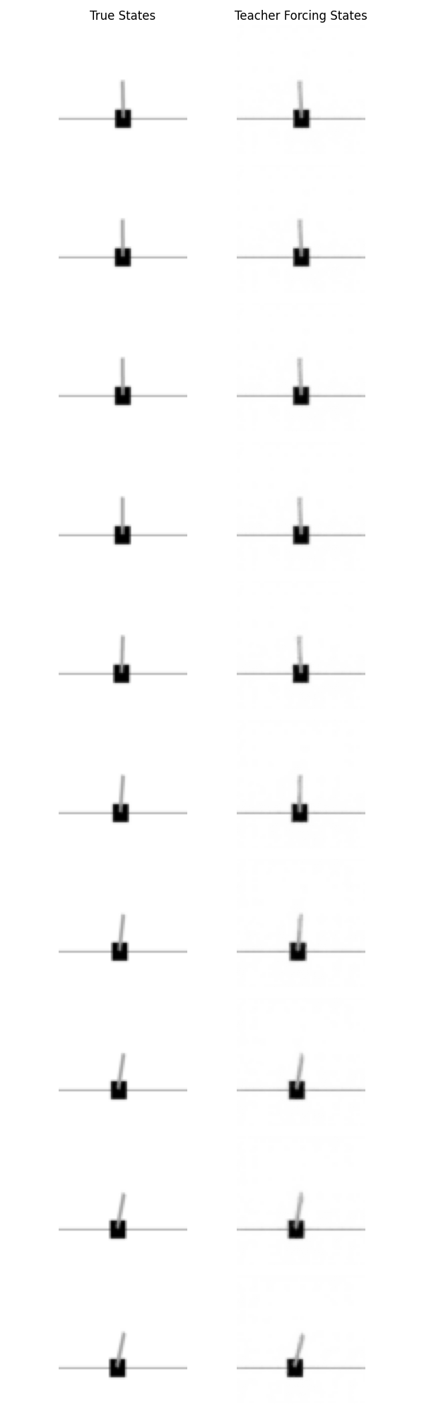
Teacher forcing
At each step, the dynamics model receives the true current latent $z_t$ from the encoder and predicts the next latent.
\[z_t \text{ (true)} \xrightarrow{M} \hat{z}_{t+1}\]This is a one-step prediction test.
If teacher forcing loss is low, then the model knows how to make local predictions from real states.
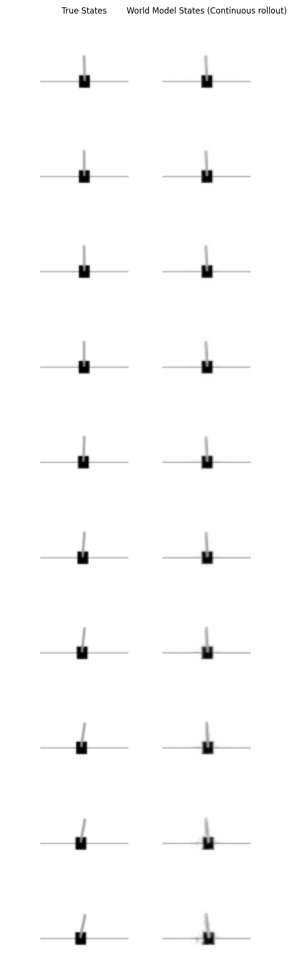
Free rollout
At each step, the dynamics model receives its own previous prediction.
\[\hat{z}_t \xrightarrow{M} \hat{z}_{t+1} \xrightarrow{M} \hat{z}_{t+2} \xrightarrow{M} \cdots\]This is the actual imagination setting. Now any small error in one step gets fed into the next step, so mistakes can accumulate. Result shows:
- teacher forcing loss stayed low
- rollout loss increased over time
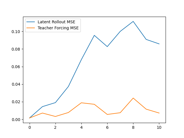
Inference: one-step prediction is good, but free-running rollout drifts. This result is not surprising, but it is important. It means the model is locally accurate but not globally stable.
If the model makes a small error at step 1, then at step 2 it is already predicting from a slightly incorrect state. That new prediction is a little worse. After a few steps, the model is operating on latent states that do not correspond to anything it saw during training, and the trajectory diverges. This is often called compounding error or temporal drift and is probably the single most useful diagnostic I got from the whole project.
What the experiments support is:
1. The latent representation is meaningful
A controller trained on $z$ can learn a useful policy. So $z$ is not just a reconstruction artifact.
2. The dynamics model is locally accurate
Teacher forcing stays low. So the dynamics model learned a real one-step approximation to the latent transitions.
3. The imagined future is unstable over time
Free rollouts drift. So this is not yet a strong long-horizon simulator.
Possible next steps:
I did not solve long-horizon latent planning, mainly due to lack of time to work on this. I also did not push the system through the standard fixes for drift, such as:
- multi-step dynamics training,
- temporal encoders,
- noise-robust latent training,
- recurrent latent states.
Solutions could be:
- Temporal latent state: Ecode two consecutive frames instead of one. That should help the model infer velocity information.
- Multistep dyanmics loss: Train the model for more than just one-step prediciton, evaluate loss on short 3-5 step rollouts during training itself. This will require a deeper model, and an more training time.
References and Further Reading:
A good repo for all things related to world modeling: https://github.com/nik-55/world-models?tab=readme-ov-file
-
Assran, Mahmoud, et al. “Self-supervised learning from images with a joint-embedding predictive architecture.” Proceedings of the IEEE/CVF conference on computer vision and pattern recognition. 2023. https://openaccess.thecvf.com/content/CVPR2023/html/Assran_Self-Supervised_Learning_From_Images_With_a_Joint-Embedding_Predictive_Architecture_CVPR_2023_paper.html ↩
-
Assran, Mido, et al. “V-jepa 2: Self-supervised video models enable understanding, prediction and planning.” arXiv preprint arXiv:2506.09985 (2025). https://arxiv.org/abs/2506.09985 ↩
-
Ha, David, and Jürgen Schmidhuber. “World models.” arXiv preprint arXiv:1803.10122 2.3 (2018): 440. https://arxiv.org/abs/1803.10122 ↩
-
Hafner, Danijar, et al. “Learning latent dynamics for planning from pixels.” International conference on machine learning. PMLR, 2019. https://icml.cc/media/icml-2019/Slides/5147.pdf ↩