The goal of this article is to make the basics of interpretability easier to understand. Feature visualization is one step towards that. It is meant to be a short summary of the key ideas highlighted by C. Olah et al. in Feature visualization¹.

Introduction

We know that a neural network optimizes its weights and biases through backpropagation. Backprop is an application of derivatives in neural networks where the gradient of the loss function with respect to each weight is calculated by propagating the error backward through the network.

In contrast to that, feature visualization uses the same gradients to modify the input data to maximize the activation of one specific neuron or layer of neurons.

Optimization

This is the step where we generate an image that activates a particular neuron/ layer in a network. Instead of starting with real images and checking for each one, we start with just a grid of noise and optimize the noisy grid with gradient ascent to make the chosen neurons fire as strongly as possible.

A good example of this is DeepDream, where the objective was to find images that a whole layer finds interesting².

Neurons may also fire for things that appear similar to the neuron but are not. For example, a particular group may show high activation for baseballs and car tire rims. The only similarity between them is that they may have the same visual pattern of stripes on them. This does not mean that pictures of baseballs or tires cause the neurons to activate, but rather, it is the pattern present in them that does. However, there is still a correlation between the images and the neurons firing. Therefore, instead of going through a dataset to find images that activate a neuron, it is better to find patterns and artifacts that do the same.

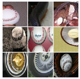
Example Image — All of these images activate the same neuron layers [1].

But there’s a problem. We now know that some neurons activate with stripes. Instead, the question we should be asking is, do these neurons only activate with stripes? A single neuron or layer in a neural network can respond to multiple different patterns, but traditional optimization methods often result in only one specific pattern being discovered. This means that multiple diverse patterns could activate the same neuron, but optimization tends to find only one of them. The solution is exploring diversity.

Diversity

It’s easier to think of diversity as a parabolic curve. A particular feature (for example, stripes) activates a neuron maximally, but that does not mean that it’s the only thing the neuron reacts to. Other points on the parabolic curve also have high activations. Not the highest maybe, but still worthy of note. These other points on the curve/ features help us understand more things that the neuron layer is reacting to. These adjacent features are created with a ‘diversity term’ that is added while the noise image is being optimized. From one noise block, now we not only have an optimized image that activates the neurons but also a second image that activates the neurons but is different from the first. The diversity term is implemented by calculating the Gram Matrix³ and then minimizing the pairwise cosine similarity⁴.

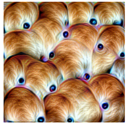
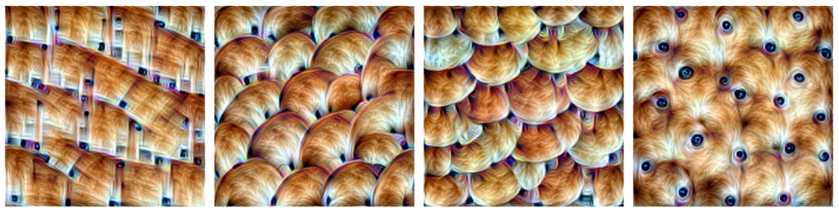
Each image is similar, and activates the same neurons, but has slightly different features (up/down arcs, circles/squares). Therefore, we now know that the neurons not only activate when shown the upward arcs but in general when shown a brown, fur-like texture¹.

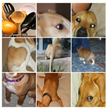
When tested on real images, the same neurons activate for fur/ brown dogs.

Activation Space

In real neural networks within our brain, images are not represented by a single neuron, but rather a group of neurons. There is evidence that combinations of neurons work together to represent images in the brain’s neural networks⁵. Much like artificial neural networks, there is also a hierarchy in biological networks. Lower-level brain regions extract basic features such as line length, and angle. Mid regions extract slightly more complex information such as movement direction, color, and shapes within the image. The higher-level regions represent more abstract information such as actual item categories and identities of things in the image. This is what allows your brain to look at a picture and say, ‘That’s a tiger in a forest’⁶. An activation space is a geometric representation of all possible combinations of neuron activations in a neural network. It has as many dimensions as there are neurons in the layer being considered. Try to think of activation space as a multi-dimensional map of how neurons in a neural network can fire together. If you had a network with just two neurons, you could plot all possible combinations of their activations on a 2D graph. With three neurons, you’d need a 3D graph. For real neural networks with many neurons, we need to imagine a space with many more dimensions. With an example of 4 neurons, if you wanted to reach a point in that space you would need to define a vector of 4 coordinates [x,y,z,w]. This framing helps us understand the concept of combining neuron activations as ‘vectors in an activation space’. Now, in this context, a basis vector would be a vector where only a single neuron fires while all other neurons are not firing i.e., [x,0,0,0].

Common sense may make us feel that a basis vector ‘firing’ might give us more information about what artifact that particular neuron is activated by. While there is evidence to support both for and against⁷ that statement, it is largely accepted to be correct as proved here⁸ and then again here¹.

The cheating network

Many times, instead of optimizing for recognizable patterns, like eyes/textures/shapes the network exploits the optimization and creates a checkerboard-like high-frequency noisy image. This is related to adversarial examples, where tiny, unnatural changes to an image can cause a neural network to misclassify it. The goal is to generate diverse patterns that neurons would respond to. But if we optimize images with no constraints we get adversarial like noise instead of meaningful diversity. These may look diverse mathematically but may not be meaningful in real-world data. The most well-known method to limit this is regularization which are primarily three types. Frequency penalization: reduce high-frequency noise⁹, Image Transformations: Translate/ Rotate/ Scale the images to prevent overfitting to artifacts, and Learned Priors: Using generative models or natural image constraints to ensure the patterns look realistic. This means that we train a model on real images, and then during optimization, we constrain the generated images to look more like the real images. This makes the generated visualizations more photorealistic and interpretable because the optimization process is not completely free to exploit network artifacts¹⁰.

Conclusion

In computational neuroscience, we analyze how real neurons encode sensory inputs and form feature representations in the brain. Feature visualization in deep learning serves a similar role: it helps us understand what artificial neurons in a neural network are detecting at different layers. Understanding either of them is beneficial to understanding the other. A simple parallel is how early layers of a CNN detect edges and textures (like V1 neurons) while deeper layers detect more complex patterns. The surprising thing is that we did not explicitly design artificial networks to behave this way, all we know is they do. In the context of image generation, one effective preconditioning method is to perform gradient descent in the Fourier domain. By transforming the image into its frequency components and scaling these frequencies to have equal energy (a process known as whitening), the optimization process can be guided to avoid undesirable high-frequency artifacts and focus on more meaningful structures¹¹.

References used in this article:

Olah, et al., “Feature Visualization”, Distill, 2017. ↩ ↩² ↩³
Mordvintsev, Alexander, Christopher Olah, and Mike Tyka. “Inceptionism: Going deeper into neural networks.” Google research blog 20.14 (2015): 5. ↩
Gram matrix, Wikipedia, Wikimedia Foundation, https://en.wikipedia.org/wiki/Gram_matrix Accessed 2/2/2025 ↩
Cosine Similarity, Wikipedia, Wikimedia Foundation https://en.wikipedia.org/wiki/Cosine_similarity Accessed 2/2/2025 ↩
How does our brain create a coherent image when we look at different objects?, Netherlands Institute for Neuroscience - Master the Mind, Accessed 2/2/2025 ↩
Roelfsema PR. Solving the binding problem: Assemblies form when neurons enhance their firing rate—they don’t need to oscillate or synchronize. Neuron. 2023;111(7):1003-1019. doi: 10.1016/j.neuron.2023.03.016 ↩
Szegedy, C. “Intriguing properties of neural networks.” arXiv preprint arXiv:1312.6199 (2013). ↩
Bau, David, et al. “Network dissection: Quantifying interpretability of deep visual representations.” Proceedings of the IEEE conference on computer vision and pattern recognition. 2017. ↩
Mahendran, Aravindh, and Andrea Vedaldi. “Understanding deep image representations by inverting them.” Proceedings of the IEEE conference on computer vision and pattern recognition. 2015. ↩
Nguyen, Anh, et al. “Synthesizing the preferred inputs for neurons in neural networks via deep generator networks.” Advances in neural information processing systems 29 (2016). ↩
Mordvintsev, et al., “Differentiable Image Parameterizations”, Distill, 2018. ↩

The goal of this article is to make the basics of interpretability easier to understand. Feature visualization is one step towards that. It is meant to be a short summary of the key ideas highlighted by C. Olah et al. in Feature visualization1.